Remote Sensing process is very significant to keep watch on earth surface features including both man-made and natural. Satellite image acquired and processed in image processing software to create spatial data. These spatial data can be further used as input data in different mathematical models to analyze the change and to find trends in future for policy planning and implementation.
GIS software also used to create input data and those spatial data can further integrated in models to analyze current as well as future scenario. GIS has many functions and tools which can be employ to find the impact in that area as well as to analysis impact of neighborhood or vice versa.
In this scenario analysis, the urban area has been re-simulated for 2015 and 2025 by including commercial and industrial areas proposed in the 2025 land use plan. The aim of this analysis is to ascertain the impacts of commercial and industrial areas on urban change.
The variable proximity to commercial and industrial areas has been created using the proposed land use plan for 2025 and is used as an input variable in the simulation model for predicting urban change for 2015 and 2025. This simulated data are analyzed with inclusion of proximity variable, termed as with inclusion (w/i) and also analyzed by excluding the above variable, termed as without inclusion (w/o).
For further analysis of simulated urban data, different zones based on distance (such as urban change within 250m, 250–500m, and 500–750m distance from proposed commercial and industrial areas) have been created for the proposed commercial and industrial classes to explore the impact of proximity to commercial and industrial activities on urban change.
These zones are categorized as zone1 (less than 250m), zone2 (between 250 and 500m), and zone3 (between 500 and 750m).
To analyze the urban change, landscape metrics are used for these simulated data. The aim of using metrics is to assess the absolute size, relative size, and complexity of urban area in these three zones.
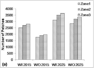
The absolute size has been described by the number of patches metrics. The number of patches metrics is expected to increase during periods of rapid urban nuclei development, but may decrease if urban areas expand and merge.
Relative size is described by the mean patch area and patch area coefficient of variation.
The mean urban patch area is a function of the number of urban patches and the size of each urban area—if the mean patch area decreases, then it implies that new urban centers are growing faster than existing urban areas. The patch size coefficient of variation is a normalized metric of the urban area.
Edge density (ED) increases with new urban nuclei, but decreases with the merging and fusing of urban areas.
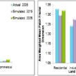
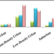
Area Weighted Mean Patch Fractal Dimension(AWMPFD) describes the shape of the urban area, which describes the complexity of urban growth.
Results of these metrics analyses are presented in below figures. Each plot represents the individual metrics in all the three zones. The increment in the number of patches metrics indicates new urban nuclei development. The numbers of patches are more in the simulated data with inclusion (w/i) compared to without inclusion (w/o) for all the zones in 2015 and 2025. All the three zones have similar trends for numbers of patches.
The difference between simulated w/i and w/o data for 2015 in zone1 is 722 patches, which is reduced to 200 patches in both types of simulated data of 2025.
The difference between both types of data for 2015 and 2025 is 699 patches and 300 patches, respectively, in zone2, but increases to 820 in 2015, and decreases to 280 in 2025 in zone3. This increase in the number of patches implies an increment in the rate of new urban nuclei development in all three zones for both periods (Figure a).

When the number of urban patches and the mean urban patch area are evaluated together, they provide a platform to understand urban area change graphically. Figure b indicates that simulated w/i have more new urban centers compared to simulated w/o data for both periods, as simulated w/o data represent higher values in all zones.
All the zones show the same trend for both periods of data and in both cases; importantly, however, the mean patch area values are decreasing as distance is increasing.
This indicates high growth of new urban developments within the 750m distance from commercial and industrial areas, especially for simulated w/i data. The numbers of patches declined while the mean patch area increased for simulated w/o data compared to simulated w/i data for both periods.
This verifies that urban growth will occur through expansion of extant urban areas rather than through spontaneous and separate development (Figure b).

The patch area coefficient of variance provides a measure of the variation within the urban area. Figure c indicates the decrease in variance between simulated w/i data and simulated w/o data for both periods in all the zones. Simulated data show that all zones reveal a slow increase in the variation within urban areas followed by a decline in variance especially in zone2.
There is a variation in values of zone3 in both types of data for both periods unlike the other two zones (Figure c).

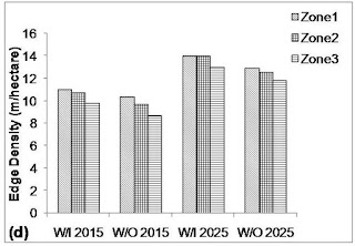
ED value is increasing with time and indicates an increase in the urban area. Simulated w/i data has higher ED values compared to simulate w/o data for both periods. ED values are higher for zone1 in both periods for all data compared to the other two zones.
Both simulated data represent increases in ED, indicating the development of a new urban area within 750m distance from commercial and industrial areas. ED values are highest for simulated w/i for 2025 in zone1 and lower for simulated w/o data for 2015 in zone3 (Figure d).
AWMPFD varied significantly among all the zones (Figure e). The simulated w/i data have more irregularity compared to simulated w/o data in zone1. Zone2 has a pattern similar to zone1’s but the shape of its urban area is less irregular when compared to zone1. AWMPFD values in zone3 have higher values compared to zone2 for both types of simulated data of 2015, which indicates greater irregularity in shape.

Simulated data for 2025 in zone3 has lower value than those of zone2 and zone1, which fact indicates a more regular shape compared to zone2 and zone1. AWMPFD indicates that zone1 has the highest complexity in its shape for all simulated data compared to the other two zones. This trend of AWMPFD indicates that complexity increased with zone1 and then decreased with zone2 and zone3 (Figure e).